Census Geography
Paul L. Delamater
Odum Institute
February 26, 2024
Overview
From the US Census Bureau’s website:
Geography is central to the work of the Census Bureau, providing the framework for survey design, sample selection, data collection, tabulation, and dissemination. Geography provides meaning and context to statistical data.
Geographic Organization
The US Census collects, estimates, and makes data available at a broad range and type of geographic units. These generally fall into two categories, enumeration units and non-enumeration units. Enumeration units are those used in the counting process for the decennial census; other units are used for a variety of purposes including (but not limited to) national and local legislative representation, legal and administrative definitions (e.g., cities and towns, school districts), and statistics (urban/rural, core based statistical areas).
If we think about the various ways in which a larger region (e.g., the US) can be subdivided into smaller units, it is important to consider the concept of hierarchy (or nesting) at various geographic scales. For example, states boundaries nest perfectly in the US (setting aside for a moment territories and sovereign nation regions)… all the places in the larger region belong to exactly one state; no places belong to 0 states or more than 1 state. At a smaller geographic level, counties (or county-like entities) nest perfectly within states… all places in a state are in exactly one county. Importantly, relating to the idea of hierarchy, no counties are located in more than one state… every county is located only within its state.
The following image (original reference) shows how US Census geographic entities are organized, illustrating which entities fit hierarchically within other entities.
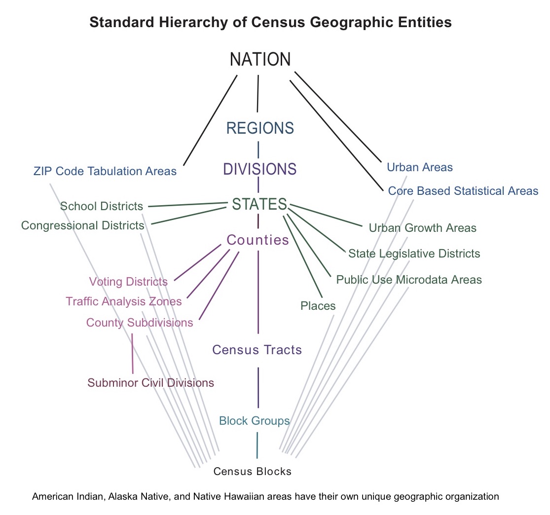
Note that the base entity is the Census Block. These are very small geographic units that were originally conceptualized as representing a “city block.” They are the building blocks of almost all other Census data. The other thing that is extremely important to note in this diagram are the entities that are not nested, for example the intermediate enumeration units (Block Groups and Tracts) do not nest perfectly within other entities such as School Districts, Congressional Districts, or Urban Areas. As an end user of US Census data, you should have a working knowledge of how the various entities are organized, because this will determine the amount of data processing you will have to perform if you end up working with non-nested entities!
The US Census provides a very long and thorough reference manual on the various geographic areas/entities. If you are interested in learning more, start with Chapters 1 and 2!
GEOID Structure
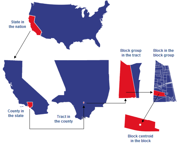
Every US Census block is assigned a 15 digit GEOID value; this is a unique identifier for every block. All the enumeration units nest within each other: blocks nest within block groups, which nest within tracts, which nest within counties, which nest within states. These relationships are stored inside the structure of the unique GEOID value.
Block GEOID
482012231001050

State is the first two digits
48

County is the next three digits (this is also known as FIPS!)
48201

Tract is the next six digits
48201223100

Block Group is the next digit
482012231001

Block is the last three digits
482012231001050
Example showing nested geographic enumeration units from https://learn.arcgis.com/en/related-concepts/GUID-D7AA4FD1-E7FE-49D7-9D11-07915C9ACC68-web.png
This information may not seem that useful, but it allows for aggregation to different geographic units without the need for spatial processing. For example, given a table with population by block, it is very straightforward to create a new table with block group, tract, or county populations.
Geographic Boundary Changes
If you are conducting a longitudinal study or a change detection analysis using US Census data, one of the more difficult aspects can be dealing with changes in the underlying geographic units (e.g., when a county or tract changes name or a set of boundaries are reconfigured). The boundaries of states do not change, however counties (and county-like entities) change every once in a while (which often necessitates changes in tracts, block groups, and blocks). The difficulty lies in that many (most?) census data sources do not revise past data to reflect these updates, thus the end user is responsible.
For example, the ACS updates their yearly data releases based on the configuration of boundaries on January 1st of that year. The US Census provides a relatively easy to read and understand summary of ACS geography; Chapter 2 is an extremely helpful one-page summary of geographic boundaries used by the ACS. The good news is that the changes are all provided in one place. The year-to-year changes in geographic units used by the ACS are provided by year on the Census website. The bad news is that there are no (to my knowledge) tables or relationship files that allow for automated normalization of ACS data using different years (thus users must deal with them on a case by case basis). However, an additional piece of good news is that the number and magnitude of the year-to-year changes are relatively small, and many users will be blissfully unaware that anything changed (because no changes occurred in their study area)!
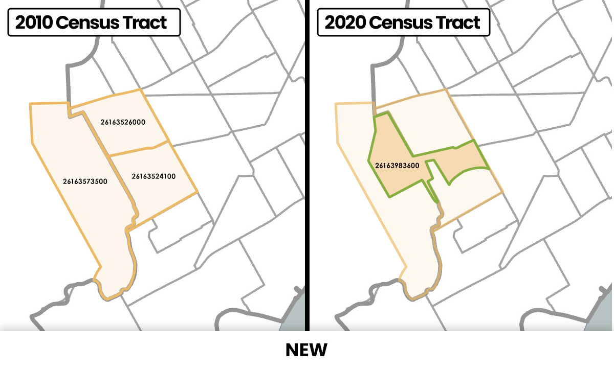
The decennial census data is accompanied by relatively large updates to the enumeration units, mainly to the number and configuration of the blocks, block groups, and tracts. These updates can be quite jarring if you are not expecting them! They are due to the nature of their use (enumeration) and are made to accomodate changes in the underlying distribution of the population. Fortunately, the US Census provides a set of relationship files that can be used to convert between consecutive decennial censuses (e.g., from 2010 to 2020) and can be used to convert data between some non-nested units (e.g., ZIP Code Tabulation Areas (ZCTAs) to tracts) in the same year. A relationship file is roughly a “crosswalk” table.
The author of tidycensus created a
function to help deal with this when working with Census data. It
uses high-resolution Census block population to re-allocate values from
one set of units to another. It is a good algorithm, but please use with
caution and make sure to check your results before using in any
analyses!
Common Boundary Changes
The following set of graphics are from https://datadrivendetroit.org/blog/2021/09/16/2020-census-tract-changes/ (this site includes a nice explanation of why these changes are important). They illustrate common changes that one might encounter when using ACS (or decennial census) data from two different time periods.


Spatial Data
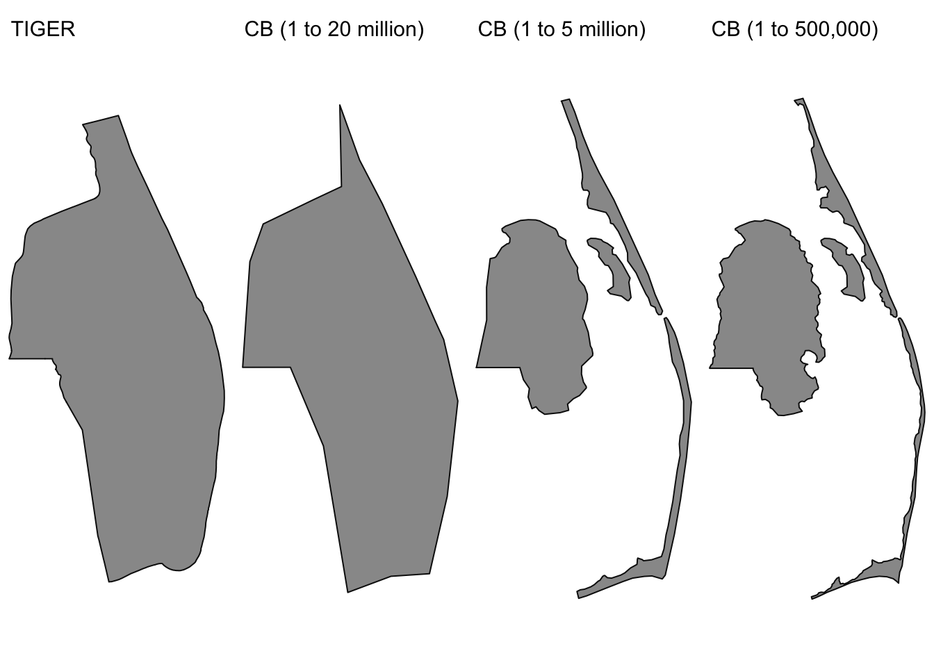
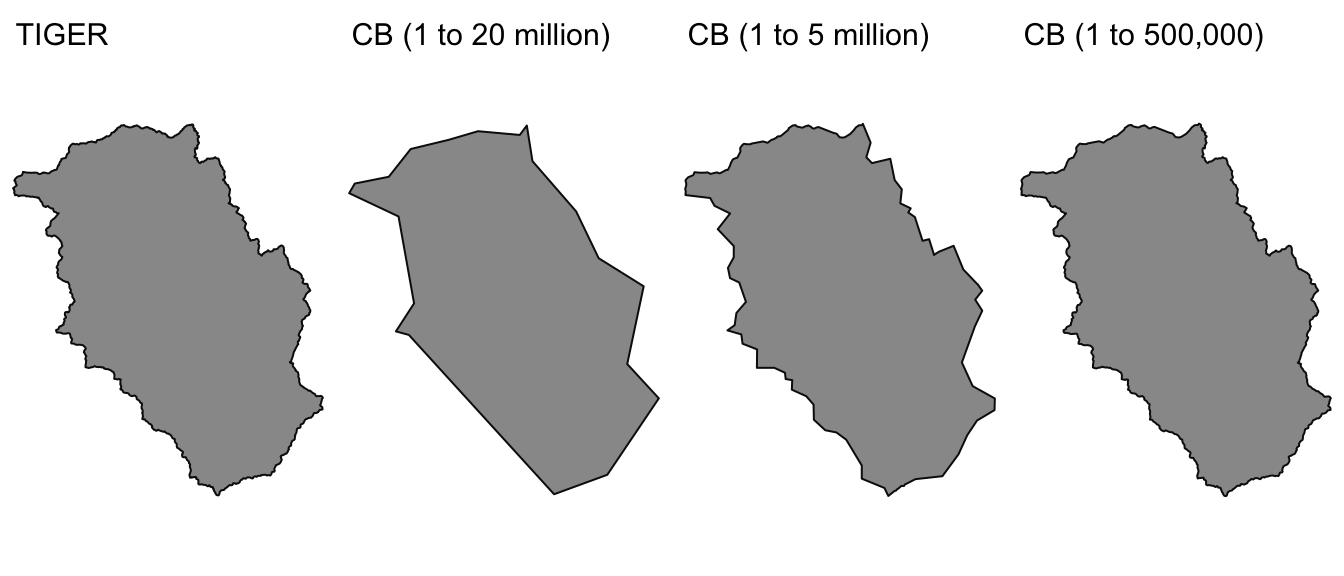
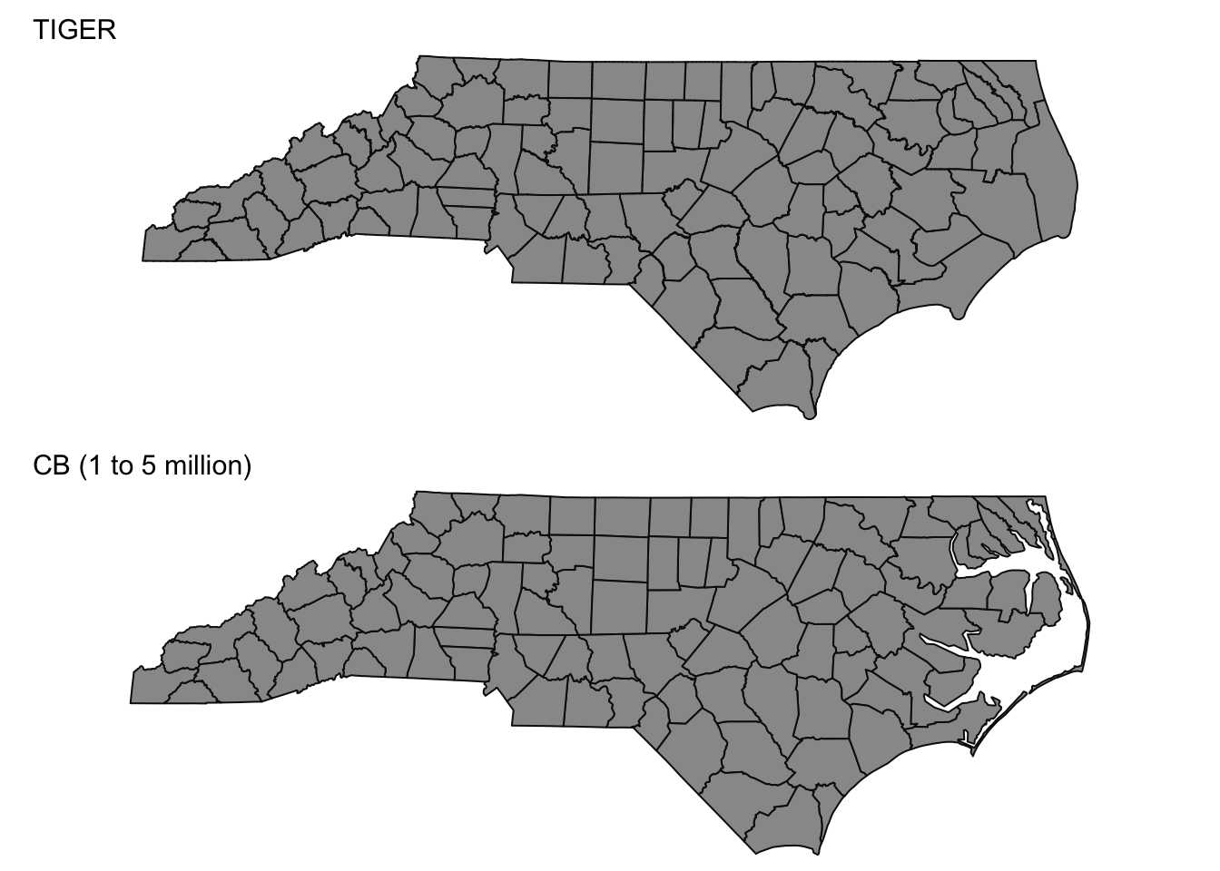
There are two types of spatial data files made available from the US Census, 1) TIGER/Line files and 2) Cartographic Boundary Files. The raw spatial data layers from the US Census do not include any demographic data, thus this information must be joined to the data!
TIGER stands for the Topologically Integrated Geographic Encoding and Referencing system and represents the U.S. Census Bureau’s “official” geographic spatial data. The correspond to legal boundaries, which can include water area (and thus may not be suitable for mapping purposes!).
Cartographic boundary files are simplified representation of selected geographic unit to be used only for display purposes (mapping). From the US Census site](https://www.census.gov/programs-surveys/geography/technical-documentation/naming-convention/cartographic-boundary-file.html):
When possible, generalization is performed with intent to maintain the hierarchical relationships among geographies and to maintain the alignment of geographies within a file set for a given year. To improve the appearance of shapes, areas are represented with fewer vertices than detailed TIGER/Line equivalents. Some small holes or discontiguous parts of areas are not included in generalized files.
While the cartographic boundary files offer advantages including improved display and smaller files, the Census warns against using them for area or perimeter calculation, geocoding, or determining precise geographic area relationships.
Example showing different spatial data layers for Dare County, North Carolina: TIGER/Line and Cartographic Boundary files for 1:20,000,000, 1:5,000,000, and 1:500,000
Example showing different spatial data layers for Yancey County, North Carolina: TIGER/Line and Cartographic Boundary files for 1:20,000,000, 1:5,000,000, and 1:500,000
Example showing different spatial data layers for North Carolina counties: TIGER/Line and 1:5,000,000 Cartographic Boundary file
This page was last updated on February 26, 2024