Overview

Preprocessing includes the (often numerous) tasks that need to be completed to prepare data for analysis. While not the most exciting part of your overall analysis, these operations are the backbone that your data and project are built upon. They can also take up a large amount of your time, so (hopefully) this module will provide you with some tools to get started on your own analysis.

### Load packages
library(tidycensus)
library(tmap)
library(tigris)
library(tidyverse)
library(sf)
library(magrittr)

### Load API key
census_api_key("YOUR API KEY GOES HERE")

Wrangling

Some of the most important but overlooked steps necessary to perform analysis in R are simple, straightforward data cleaning and management tasks. The following set of commands walks through the process of some common steps required to prepare your data for analysis.

### Retrieve Race/Ethnicity data
### Search for B03002 in ACS2020_Table_Shells.xlsx
### Note the hierarchy (nesting of groups)
wayne_acs5_2020_re <- get_acs(state = "MI",
                              county = "Wayne",
                              geography = "tract",
                              table = "B03002",
                              year = 2020,
                              survey = "acs5",
                              output = "wide",
                              geometry = TRUE)

###
### Use select to only keep certain columns
### 
wayne_example <- wayne_acs5_2020_re %>% select(GEOID, NAME)

### Discard the Name and Margin of Error columns
### Select GEOID and cols that end with E
### Do not select NAME
wayne_acs5_2020_re %<>% select(GEOID, ends_with("E"), -c(NAME))

### Rename columns
wayne_acs5_2020_re %<>% rename(TOTAL_POP = B03002_001E,
                               NH_POP = B03002_002E,
                               HISP_POP = B03002_012E,
                               NH_WHITE_POP = B03002_003E,
                               NH_BLACK_POP = B03002_004E,
                               NH_AIAN_POP = B03002_005E,
                               NH_ASIAN_POP = B03002_006E,
                               NH_NHPI_POP = B03002_007E,
                               NH_OTHER_POP = B03002_008E,
                               NH_TWO_POP = B03002_009E)

### Subset columns and reorder
wayne_acs5_2020_re %<>% select(GEOID, TOTAL_POP:NH_POP, NH_WHITE_POP:NH_TWO_POP, HISP_POP)

### Preview
glimpse(wayne_acs5_2020_re)

## Rows: 627
## Columns: 12
## $ GEOID        [3m[38;5;246m<chr>[39m[23m "26163583200", "26163562400", "26163541500", "26163507400", "26163584400", "26163564300", "26163556900", "…
## $ TOTAL_POP    [3m[38;5;246m<dbl>[39m[23m 2231, 5252, 4020, 2135, 2727, 2376, 3767, 5227, 3792, 5312, 2137, 2595, 2838, 1982, 4513, 5377, 1906, 1503…
## $ NH_POP       [3m[38;5;246m<dbl>[39m[23m 2171, 5252, 4020, 2087, 2590, 2276, 3671, 5213, 3792, 4877, 2103, 2374, 2451, 1982, 4181, 5348, 1775, 1498…
## $ NH_WHITE_POP [3m[38;5;246m<dbl>[39m[23m 1859, 4778, 44, 25, 1923, 1839, 2937, 16, 57, 4551, 1913, 2245, 1616, 89, 3947, 5043, 1263, 0, 136, 3465, …
## $ NH_BLACK_POP [3m[38;5;246m<dbl>[39m[23m 107, 128, 3890, 2043, 402, 173, 83, 5164, 3660, 244, 63, 10, 749, 1880, 166, 266, 374, 1498, 3700, 18, 126…
## $ NH_AIAN_POP  [3m[38;5;246m<dbl>[39m[23m 0, 0, 28, 0, 17, 0, 0, 33, 0, 8, 0, 0, 0, 0, 0, 0, 0, 0, 9, 0, 4, 0, 9, 10, 0, 0, 25, 0, 0, 0, 0, 0, 0, 7,…
## $ NH_ASIAN_POP [3m[38;5;246m<dbl>[39m[23m 14, 266, 0, 0, 55, 249, 600, 0, 0, 0, 89, 0, 42, 0, 21, 0, 20, 0, 1, 0, 208, 17, 0, 2, 0, 1175, 0, 0, 0, 0…
## $ NH_NHPI_POP  [3m[38;5;246m<dbl>[39m[23m 0, 0, 0, 0, 0, 0, 0, 0, 0, 0, 0, 0, 0, 0, 0, 0, 0, 0, 0, 0, 0, 0, 0, 0, 0, 0, 0, 0, 0, 0, 0, 0, 0, 0, 0, 0…
## $ NH_OTHER_POP [3m[38;5;246m<dbl>[39m[23m 23, 30, 0, 19, 0, 0, 0, 0, 25, 0, 0, 0, 0, 11, 16, 0, 9, 0, 0, 0, 0, 0, 0, 0, 2, 0, 0, 59, 0, 0, 23, 0, 30…
## $ NH_TWO_POP   [3m[38;5;246m<dbl>[39m[23m 168, 50, 58, 0, 193, 15, 51, 0, 50, 74, 38, 119, 44, 2, 31, 39, 109, 0, 39, 168, 78, 0, 3, 0, 135, 38, 196…
## $ HISP_POP     [3m[38;5;246m<dbl>[39m[23m 60, 0, 0, 48, 137, 100, 96, 14, 0, 435, 34, 221, 387, 0, 332, 29, 131, 5, 28, 244, 679, 0, 88, 8, 130, 192…
## $ geometry     [3m[38;5;246m<MULTIPOLYGON [°]>[39m[23m MULTIPOLYGON (((-83.30828 4..., MULTIPOLYGON (((-83.50904 4..., MULTIPOLYGON (((-83.26851 4..…

Calculate Percents

The data downloaded from the Census comes as counts. For some analyses and visualizations counts are appropriate; however, for many others, working with proportions or percents is a much better option. The following example shows how to divide a set of contiguous columns by a single column. Be careful with commands such as these!… they’re easy to get wrong.

### Make a copy of object to work with
wayne_acs5_2020_re_p <- wayne_acs5_2020_re

### Use indexing to select set of columns
### New, purrr style function
wayne_acs5_2020_re_p %<>% mutate(across(c(HISP_POP:NH_TWO_POP), ~ . / TOTAL_POP))

### Preview
glimpse(wayne_acs5_2020_re_p)

## Rows: 627
## Columns: 12
## $ GEOID        [3m[38;5;246m<chr>[39m[23m "26163583200", "26163562400", "26163541500", "26163507400", "26163584400", "26163564300", "26163556900", "…
## $ TOTAL_POP    [3m[38;5;246m<dbl>[39m[23m 2231, 5252, 4020, 2135, 2727, 2376, 3767, 5227, 3792, 5312, 2137, 2595, 2838, 1982, 4513, 5377, 1906, 1503…
## $ NH_POP       [3m[38;5;246m<dbl>[39m[23m 2171, 5252, 4020, 2087, 2590, 2276, 3671, 5213, 3792, 4877, 2103, 2374, 2451, 1982, 4181, 5348, 1775, 1498…
## $ NH_WHITE_POP [3m[38;5;246m<dbl>[39m[23m 1859, 4778, 44, 25, 1923, 1839, 2937, 16, 57, 4551, 1913, 2245, 1616, 89, 3947, 5043, 1263, 0, 136, 3465, …
## $ NH_BLACK_POP [3m[38;5;246m<dbl>[39m[23m 107, 128, 3890, 2043, 402, 173, 83, 5164, 3660, 244, 63, 10, 749, 1880, 166, 266, 374, 1498, 3700, 18, 126…
## $ NH_AIAN_POP  [3m[38;5;246m<dbl>[39m[23m 0, 0, 28, 0, 17, 0, 0, 33, 0, 8, 0, 0, 0, 0, 0, 0, 0, 0, 9, 0, 4, 0, 9, 10, 0, 0, 25, 0, 0, 0, 0, 0, 0, 7,…
## $ NH_ASIAN_POP [3m[38;5;246m<dbl>[39m[23m 14, 266, 0, 0, 55, 249, 600, 0, 0, 0, 89, 0, 42, 0, 21, 0, 20, 0, 1, 0, 208, 17, 0, 2, 0, 1175, 0, 0, 0, 0…
## $ NH_NHPI_POP  [3m[38;5;246m<dbl>[39m[23m 0, 0, 0, 0, 0, 0, 0, 0, 0, 0, 0, 0, 0, 0, 0, 0, 0, 0, 0, 0, 0, 0, 0, 0, 0, 0, 0, 0, 0, 0, 0, 0, 0, 0, 0, 0…
## $ NH_OTHER_POP [3m[38;5;246m<dbl>[39m[23m 23, 30, 0, 19, 0, 0, 0, 0, 25, 0, 0, 0, 0, 11, 16, 0, 9, 0, 0, 0, 0, 0, 0, 0, 2, 0, 0, 59, 0, 0, 23, 0, 30…
## $ NH_TWO_POP   [3m[38;5;246m<dbl>[39m[23m 0.075302555, 0.009520183, 0.014427861, 0.000000000, 0.070773744, 0.006313131, 0.013538625, 0.000000000, 0.…
## $ HISP_POP     [3m[38;5;246m<dbl>[39m[23m 0.026893770, 0.000000000, 0.000000000, 0.022482436, 0.050238357, 0.042087542, 0.025484470, 0.002678401, 0.…
## $ geometry     [3m[38;5;246m<MULTIPOLYGON [°]>[39m[23m MULTIPOLYGON (((-83.30828 4..., MULTIPOLYGON (((-83.50904 4..., MULTIPOLYGON (((-83.26851 4..…

Query (Subset)

A query is a request for information from a data table or set of features. We often use queries as a preprocessing step, as they allow us to subset our data. The following examples show non-spatial and spatial queries.

Attribute Query

An attribute query uses the data stored in the tabular portion of a spatial data layer. For example, we can subset our data from Detroit to only include Census tracts with 1 or more people residing in them. We can also use queries to find out simple information about our data.

## Number of rows (for reference)
nrow(wayne_acs5_2020_re_p)

## [1] 627

### Use filter for attribute queries
### Select tracts with population > 0
wayne_acs5_2020_re_p_gt0 <- wayne_acs5_2020_re_p %>% filter(TOTAL_POP > 0)

## Number of rows in subset
nrow(wayne_acs5_2020_re_p_gt0)

## [1] 586

## Select tracts with a large (>50%) White population and count
wayne_acs5_2020_re_p %>% filter(NH_WHITE_POP > 0.5) %>%
  nrow()

## [1] 575

## Select tracts with a large (>50%) Black population and count
wayne_acs5_2020_re_p %>% filter(NH_BLACK_POP > 0.5) %>%
  nrow()

## [1] 574

Spatial Query

A spatial query uses information from one spatial data layer to select features in another spatial data layer. A simple use for spatial queries when using Census data is to spatially subset a set of features (e.g., tracts) to a legal boundary of a, for example, municipality. Remember that enumeration units do not always nest nicely in legally defined entities such as cities and towns! However, we can leverage the spatial information in each layer to perform these operations. For example, the city of Detroit falls inside of Wayne County, MI. We can use the boundaries of Detroit to subset our tracts to only those that fall (partially or completely) inside the city. We’ll get the city boundaries from the Census using the tigris package (created by the author of tidycensus).

Example showing tract boundaries in Wayne County, MI and boundary of the City of Detroit

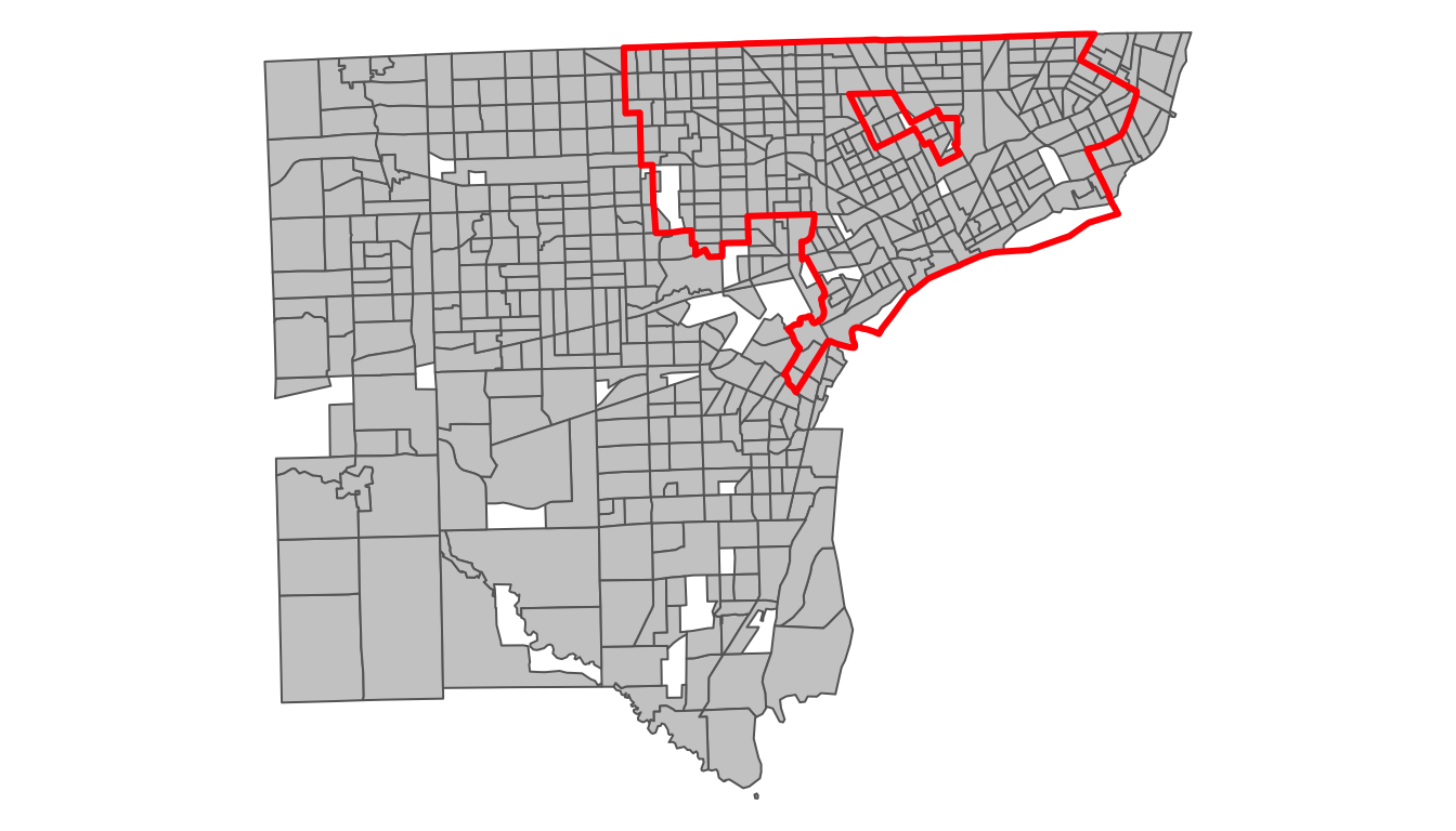
NOTE: This set of maps uses the object with tracts with 0 population removed. When creating this tutorial, I was getting an error when trying to map the entire set of polygons due to some polygons having bad geometry. This, unfortunately, happens somewhat often, especially when working with data bordering water!

## Use tigris function to get Places in Michigan
MI_places <- places(state = "MI")

## Use attribute query to subset to only Detroit
Detroit_city <- MI_places %>% filter(NAME == "Detroit")

## Use spatial filter!
Detroit_acs5_2020_re_p_gt0 <- wayne_acs5_2020_re_p_gt0 %>% st_filter(Detroit_city)

## How many tracts?
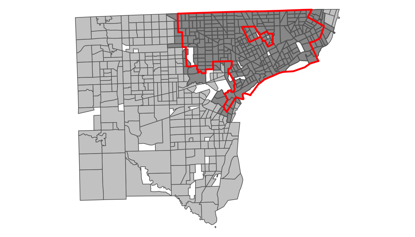
nrow(Detroit_acs5_2020_re_p_gt0)

## [1] 312

Example showing tract boundaries in Wayne County, MI and boundary of the City of Detroit (with tracts included in the Detroit subset)

Join Data

Joining or merging together data from two different sources or tables is another oft-used task in data preprocessing; it is an essential part of integrating data together. Mirroring the two types of queries, joining can be done via an operation on attributes or via a spatial overlay.

Table Join

When performing a table join, columns from one table are appended to another table based on the relationship in a common column or field in the two tables, which is called a “key” field. A key field has one extremely important property: every observation must have a unique entry. For a key field and join to function properly, observations cannot share values in the key field! In US Census data, we use the GEOID field. Although the content of the key fields must be the same in both tables, the names of the fields do not need to be the same in both tables. For example, the key field may be called “GEOID” in your ACS data and “GEOID10” in your decennial census data table. The important part is that the entries in the two fields represent the exact same thing… with the exact same entries!

Below is an example where an additional table is downloaded from the 2020 census and joined to our table with age information for Detroit.

## Get housing data for Wayne County
wayne_dec_2020_housing <- get_decennial(state = "MI",
                                        county = "Wayne",
                                        geography = "tract",
                                        table = "H1",
                                        year = 2020,
                                        sumfile = "pl",
                                        output = "wide",
                                        geometry = FALSE)

### Use a left join
### Object "receiving" data is first
Detroit_dat <- left_join(Detroit_acs5_2020_re_p_gt0,
                         wayne_dec_2020_housing,
                         by = "GEOID")

### Summary
glimpse(Detroit_dat)

## Rows: 312
## Columns: 16
## $ GEOID        [3m[38;5;246m<chr>[39m[23m "26163541500", "26163507400", "26163539200", "26163506900", "26163504300", "26163535100", "26163500900", "…
## $ TOTAL_POP    [3m[38;5;246m<dbl>[39m[23m 4020, 2135, 5227, 3792, 1982, 1503, 3913, 1949, 1620, 1356, 5499, 2544, 3866, 2757, 2694, 4052, 688, 1883,…
## $ NH_POP       [3m[38;5;246m<dbl>[39m[23m 4020, 2087, 5213, 3792, 1982, 1498, 3885, 1270, 1620, 1348, 1513, 2263, 3791, 2757, 2651, 4052, 660, 1847,…
## $ NH_WHITE_POP [3m[38;5;246m<dbl>[39m[23m 44, 25, 16, 57, 89, 0, 136, 854, 9, 36, 1036, 196, 260, 6, 484, 26, 253, 222, 317, 1577, 130, 265, 25, 131…
## $ NH_BLACK_POP [3m[38;5;246m<dbl>[39m[23m 3890, 2043, 5164, 3660, 1880, 1498, 3700, 126, 1594, 1300, 256, 1974, 3343, 2742, 1874, 3947, 392, 1441, 2…
## $ NH_AIAN_POP  [3m[38;5;246m<dbl>[39m[23m 28, 0, 33, 0, 0, 0, 9, 4, 0, 10, 25, 0, 0, 0, 0, 0, 7, 12, 0, 0, 11, 0, 0, 13, 0, 0, 7, 0, 0, 0, 0, 0, 0, …
## $ NH_ASIAN_POP [3m[38;5;246m<dbl>[39m[23m 0, 0, 0, 0, 0, 0, 1, 208, 17, 2, 0, 0, 0, 0, 248, 0, 0, 95, 0, 26, 0, 10, 0, 0, 0, 0, 0, 0, 0, 16, 0, 0, 0…
## $ NH_NHPI_POP  [3m[38;5;246m<dbl>[39m[23m 0, 0, 0, 0, 0, 0, 0, 0, 0, 0, 0, 0, 0, 0, 0, 0, 0, 0, 0, 0, 0, 0, 0, 0, 0, 0, 0, 0, 0, 0, 0, 0, 0, 0, 0, 0…
## $ NH_OTHER_POP [3m[38;5;246m<dbl>[39m[23m 0, 19, 0, 25, 11, 0, 0, 0, 0, 0, 0, 59, 0, 0, 23, 30, 0, 0, 0, 0, 0, 0, 0, 0, 0, 0, 0, 0, 0, 122, 0, 0, 0,…
## $ NH_TWO_POP   [3m[38;5;246m<dbl>[39m[23m 0.014427861, 0.000000000, 0.000000000, 0.013185654, 0.001009082, 0.000000000, 0.009966777, 0.040020523, 0.…
## $ HISP_POP     [3m[38;5;246m<dbl>[39m[23m 0.0000000000, 0.0224824356, 0.0026784006, 0.0000000000, 0.0000000000, 0.0033266800, 0.0071556351, 0.348383…
## $ NAME         [3m[38;5;246m<chr>[39m[23m "Census Tract 5415, Wayne County, Michigan", "Census Tract 5074, Wayne County, Michigan", "Census Tract 53…
## $ H1_001N      [3m[38;5;246m<dbl>[39m[23m 1794, 1206, 2313, 1459, 912, 819, 1540, 1278, 1005, 891, 1483, 1299, 1626, 1234, 2126, 1957, 127, 1490, 64…
## $ H1_002N      [3m[38;5;246m<dbl>[39m[23m 1568, 993, 2184, 1273, 702, 645, 1338, 1160, 773, 576, 1290, 1062, 1338, 993, 1940, 1824, 121, 1136, 532, …
## $ H1_003N      [3m[38;5;246m<dbl>[39m[23m 226, 213, 129, 186, 210, 174, 202, 118, 232, 315, 193, 237, 288, 241, 186, 133, 6, 354, 108, 84, 226, 34, …
## $ geometry     [3m[38;5;246m<MULTIPOLYGON [°]>[39m[23m MULTIPOLYGON (((-83.26851 4..., MULTIPOLYGON (((-83.09494 4..., MULTIPOLYGON (((-83.20052 4..…

Spatial Join

Spatial join is required to merge attributes when there is no shared attribute (key field). This type of join requires two spatial data layers and leverages the fact that all observations are georeferenced. This type of join is very popular for assigning attributes of polygons (e.g., neighborhoods) to point locations.

In the below example, hospital data from Michigan (point locations) are spatially joined to the ACS data for Wayne County. Each hospital is assigned the attributes of the census tract it is located within. Note that the data have to have the same coordinate reference system (CRS or projection) to be joined. In this example, they are different (because they are from different sources), hence the hospital data layer is reprojected to match the spatial data layer from the census.

### Read in health care facility data
MI_health_care_facs <- read_sf("https://utility.arcgis.com/usrsvcs/servers/d6ffb0eed44e416586f30a51189f276e/rest/services/CSS/CSS_LARA/MapServer/6/query?outFields=*&where=1%3D1&f=geojson")

## Use attribute query to subset to only hospitals
MI_hospitals <- MI_health_care_facs %>% filter(FacilityType == "Hospital")

## Reproject MI hospitals object to CRS of census data
MI_hospitals %<>% st_transform(st_crs(wayne_acs5_2020_re_p_gt0))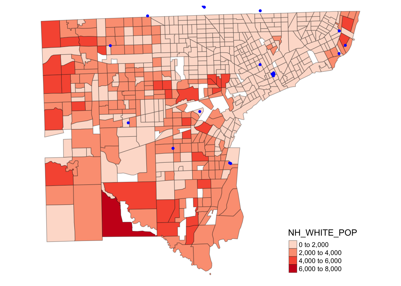

### Perform spatial join
### Object receiving attributes is listed first
Detroit_hospitals <- st_join(MI_hospitals,
                             Detroit_acs5_2020_re_p_gt0,
                             left = FALSE)  ## Only keep Detroit hospitals
                             
### Summary
glimpse(Detroit_hospitals)

## Rows: 12
## Columns: 32
## $ LicenseNumber    [3m[38;5;246m<chr>[39m[23m "1060000026", "1060000043", "1060000052", "1060000072", "1060000103", "1060000132", "1060000135", "106…
## $ FacilityTypeCode [3m[38;5;246m<chr>[39m[23m "1060", "1060", "1060", "1060", "1060", "1060", "1060", "1060", "1060", "1060", "1060", "1060"
## $ FacilityType     [3m[38;5;246m<chr>[39m[23m "Hospital", "Hospital", "Hospital", "Hospital", "Hospital", "Hospital", "Hospital", "Hospital", "Hospi…
## $ Name             [3m[38;5;246m<chr>[39m[23m "HENRY FORD HEALTH HOSPITAL", "BEAUMONT HOSPITAL, GROSSE POINTE", "HARPER UNIVERSITY HOSPITAL", "ASCEN…
## $ StreetAddress    [3m[38;5;246m<chr>[39m[23m "2799 W GRAND BLVD", "468 CADIEUX RD", "3990 JOHN R STREET", "22101 MOROSS RD", "4201 ST ANTOINE ST - …
## $ City             [3m[38;5;246m<chr>[39m[23m "DETROIT", "GROSSE POINTE", "DETROIT", "DETROIT", "DETROIT", "DETROIT", "DETROIT", "DETROIT", "DETROIT…
## $ State            [3m[38;5;246m<chr>[39m[23m "MI", "MI", "MI", "MI", "MI", "MI", "MI", "MI", "MI", "MI", "MI", "MI"
## $ Zip              [3m[38;5;246m<chr>[39m[23m "48202", "48230", "48201", "48236", "48201", "48201", "48201", "48201", "48201", "48236", "48201", "48…
## $ County           [3m[38;5;246m<chr>[39m[23m "WAYNE", "WAYNE", "WAYNE", "WAYNE", "WAYNE", "WAYNE", "WAYNE", "WAYNE", "WAYNE", "WAYNE", "WAYNE", "WA…
## $ TotalCapacity    [3m[38;5;246m<int>[39m[23m 877, 280, 470, 654, 248, 228, 69, 114, 123, 4, 28, 26
## $ ServesAdults     [3m[38;5;246m<int>[39m[23m 0, 0, 0, 0, 0, 0, 0, 0, 0, 0, 0, 0
## $ ServesChildren   [3m[38;5;246m<int>[39m[23m 0, 0, 0, 0, 0, 0, 0, 0, 0, 0, 0, 0
## $ AddressID        [3m[38;5;246m<int>[39m[23m 2833, 4443, 3955, 15956, 28269, 3896, 2637, 3954, 4074, 1263, 2636, 15957
## $ stdStreetAddress [3m[38;5;246m<chr>[39m[23m "2799 W Grand Blvd", "468 Cadieux Rd", "3990 John R St", "22101 Moross Rd", "4201 St Antoine St", "390…
## $ stdCity          [3m[38;5;246m<chr>[39m[23m "Detroit", "Grosse Pointe", "Detroit", "Detroit", "Detroit", "Detroit", "Detroit", "Detroit", "Detroit…
## $ stdState         [3m[38;5;246m<chr>[39m[23m "MI", "MI", "MI", "MI", "MI", "MI", "MI", "MI", "MI", "MI", "MI", "MI"
## $ stdZip           [3m[38;5;246m<chr>[39m[23m "48202", "48230", "48201", "48236", "48201", "48201", "48201", "48201", "48201", "48236", "48201", "48…
## $ Latitude         [3m[38;5;246m<dbl>[39m[23m 42.36640, 42.38387, 42.35138, 42.41977, 42.35343, 42.35167, 42.34869, 42.35138, 42.35153, 42.39692, 42…
## $ Longitude        [3m[38;5;246m<dbl>[39m[23m -83.08375, -82.91497, -83.05775, -82.91451, -83.05482, -83.05396, -83.05525, -83.05775, -83.05785, -82…
## $ ESRI_OID         [3m[38;5;246m<int>[39m[23m 363, 378, 387, 406, 432, 456, 458, 460, 485, 488, 492, 495
## $ geometry         [3m[38;5;246m<POINT [°]>[39m[23m POINT (-83.08375 42.3664), POINT (-82.91497 42.38387), POINT (-83.05775 42.35138), POINT (-82.91451 42…
## $ GEOID            [3m[38;5;246m<chr>[39m[23m "26163522400", "26163550400", "26163517500", "26163501600", "26163517500", "26163517500", "26163517500…
## $ TOTAL_POP        [3m[38;5;246m<dbl>[39m[23m 938, 1503, 2694, 2258, 2694, 2694, 2694, 2694, 2694, 5160, 2694, 2258
## $ NH_POP           [3m[38;5;246m<dbl>[39m[23m 920, 1481, 2651, 2229, 2651, 2651, 2651, 2651, 2651, 4989, 2651, 2229
## $ NH_WHITE_POP     [3m[38;5;246m<dbl>[39m[23m 199, 1352, 484, 368, 484, 484, 484, 484, 484, 4747, 484, 368
## $ NH_BLACK_POP     [3m[38;5;246m<dbl>[39m[23m 695, 87, 1874, 1796, 1874, 1874, 1874, 1874, 1874, 35, 1874, 1796
## $ NH_AIAN_POP      [3m[38;5;246m<dbl>[39m[23m 1, 3, 0, 0, 0, 0, 0, 0, 0, 7, 0, 0
## $ NH_ASIAN_POP     [3m[38;5;246m<dbl>[39m[23m 13, 0, 248, 0, 248, 248, 248, 248, 248, 107, 248, 0
## $ NH_NHPI_POP      [3m[38;5;246m<dbl>[39m[23m 0, 0, 0, 0, 0, 0, 0, 0, 0, 0, 0, 0
## $ NH_OTHER_POP     [3m[38;5;246m<dbl>[39m[23m 0, 0, 23, 43, 23, 23, 23, 23, 23, 0, 23, 43
## $ NH_TWO_POP       [3m[38;5;246m<dbl>[39m[23m 0.012793177, 0.025948104, 0.008166295, 0.009743136, 0.008166295, 0.008166295, 0.008166295, 0.008166295…
## $ HISP_POP         [3m[38;5;246m<dbl>[39m[23m 0.01918977, 0.01463739, 0.01596140, 0.01284322, 0.01596140, 0.01596140, 0.01596140, 0.01596140, 0.0159…

Challenge

Create an R script that contains (only) the required commands to download the 2020 ACS 5-year data for Household Income (B19001) at the tract level for Mecklenburg County, North Carolina; rename the columns (hint: do not start column names with numbers); and calculate the proportion of households in each household income class. Make sure that the data are in wide format and include the spatial features. Write out the data!

Code

Click here to download the R code from this module

This page was last updated on February 26, 2024

Preprocessing

Paul L. Delamater

Odum Institute

February 26, 2024