Spatial Analysis
Paul L. Delamater
Odum Institute
February 26, 2024
Overview
The following sections provide a few examples of analyses that can be conducted using US Census data.
### Load packages
library(tidycensus)
library(tigris)
library(tmap)
library(tidyverse)
library(sf)
library(magrittr)
library(spdep)

### Load API key
census_api_key("YOUR API KEY GOES HERE")
Spatial Analysis
Tobler’s First Law of Geography:
Everything is related to everything else, but near things are more related than distant things.
When analyzing US Census data, we may be interested in evaluating (quantitatively) whether values of a variable cluster geographically; we may also be interested in identifying where clusters of similar values are found. The following code provides an introduction to spatial cluster analysis. It is broken into two subsections, Global Spatial Autocorrelation and Local Spatial Autocorrelation. It uses the population change data from the Analysis module, which is recreated below.
### Retrieve population counts by tract for Wake County, NC
wake_dec_2020_pop <- get_decennial(state = "NC",
                                   county = "Wake",
                                   geography = "tract",
                                   variables = "P1_001N",
                                   year = 2020,
                                   sumfile = "pl",
                                   geometry = TRUE) %>% st_make_valid()
                                                    ### ^^ fixes issues in spatial layer
wake_dec_2010_pop <- get_decennial(state = "NC",
                                   county = "Wake",
                                   geography = "tract",
                                   variables = "P001001",
                                   year = 2010,
                                   sumfile = "pl",
                                   geometry = TRUE) %>% st_make_valid()

### Retrieve the block population counts for Wake County, 2020
wake_block_pop <- blocks("NC",
                         "Wake",
                         year = 2020)

### Interpolate
wake_dec_2010_pop_20 <- interpolate_pw(from = wake_dec_2010_pop,
                                       to = wake_dec_2020_pop,
                                       to_id = "GEOID",
                                       weights = wake_block_pop,
                                       weight_column = "POP20",
                                       extensive = TRUE)

## Rename population column in 2020 data
wake_dec_2020_pop %<>% rename(POP20 = value)

## Rename population column in "new" 2010 data
wake_dec_2010_pop_20 %<>% rename(POP10 = value)

## Table join population in 2010 (in 2020 tracts)
wake_dec_2020_pop %<>% left_join(wake_dec_2010_pop_20 %>% st_drop_geometry(),
                                 by = "GEOID")

## Calculate population change (raw and percent)
wake_dec_2020_pop %<>% mutate(POPCH_10_20 = POP20 - POP10,
                              POPCH_10_20pct = 100 * POPCH_10_20 / POP10)
Global Spatial Autocorrelation
Spatial autocorrelation is the formal definition of Tobler’s law. It measures how similar the values of nearby units are to one another. In this case, we will calculate a Moran’s I value for population percent change to determine whether places near to each other had similar change.
Spatial Neighbors
First, we must explicitly define which observations are located “near” to one another. In R, we create a neighborhood object to accomplish this. While there are a number of different ways to define spatial neighbors, we are going to base them on shared boundaries.
## First, remove any regions with NA for our variable of interest
## This is important when performing spatial autocorrelation analysis
wake_dec_2020_pop %<>% filter(!is.na(POPCH_10_20pct))

## Create Queen case neighbors
wake_queen <- poly2nb(wake_dec_2020_pop,
                      queen = TRUE)
Moran’s I
Moran’s I measures the magnitude and nature of spatial autocorrelation. It is a global variable, meaning that it averages over all of the observations in the data. Values range from a high of 1 (perfect clustering), to 0 (completely random), to -1 (perfect dispersion).
## First, convert our neighbors to weight matrix
wake_queen_weights <- nb2listw(
  wake_queen,
  style = "B",                  # B is binary (1,0)
  zero.policy = TRUE)           # zero.policy allows for observations with NO neighbors

# Uncomment and run for information about the neighborhoods!
# summary(wake_queen_weights, zero.policy = TRUE)

## Moran's I
wake_popch_I <- moran.test(
  wake_dec_2020_pop$POPCH_10_20pct, # The column in your sp data
  wake_queen_weights,               # Weights object
  zero.policy = TRUE,               # Allows for observations with NO neighbors
  randomisation = TRUE)             # Compares to randomized NULL data

## Print summary to screen
wake_popch_I
##
## Moran I test under randomisation
##
## data: wake_dec_2020_pop$POPCH_10_20pct
## weights: wake_queen_weights
##
## Moran I statistic standard deviate = 8.1452, p-value < 2.2e-16
## alternative hypothesis: greater
## sample estimates:
## Moran I statistic Expectation Variance
## 0.298046973 -0.004385965 0.001378655In this case, Moran’s I is nearly 0.3, which indicated moderate spatial clustering. I would interpret this as strong evidence of a larger regional pattern (spatial clustering) of population change occurring in Wake county between 2010 and 2020.
Local Spatial Autocorrelation
Measures of local spatial autocorrelation focus on identifying where spatial autocorrelation is high, low, or not existent. Instead of returning a single value for the entire dataset, these measures return a value for every observation, meaning they can be mapped.
LISA
LISA stands for Local Indicators of Spatial Association; for all intents and purposes, it is a local version of Moran’s I. However, LISA provides some very helpful information, the location of four potential types of observations: high-high spatial clusters and low-low spatial clusters, where observations are surrounded by similar values, and high/low spatial outliers, where observations are surrounded by dissimilar values.
## First, scale our data
wake_dec_2020_pop %<>% mutate(POPCH_10_20pct_sc = as.numeric(scale(POPCH_10_20pct)))

## LISA -- Local Moran's I
wake_popch_lisa <- localmoran_perm(
  wake_dec_2020_pop$POPCH_10_20pct_sc,                         # The column in your sp data
                                   wake_queen_weights,         # Weights object
                                   zero.policy = TRUE,         # Best to keep TRUE for LISA
                                   nsim = 999L,
                                   alternative = "two.sided"
) %>%
  as_tibble() %>%                                              # Make result into tibble
  set_names(c("local_i", "exp_i", "var_i", "z_i", "p_i",
              "p_i_sim", "pi_sim_folded", "skewness", "kurtosis"))

## To get "nice" LISA categories for mapping
## takes a bit of work in R, unfortunately

# Scale the input data to deviation from mean
cDV <- wake_dec_2020_pop$POPCH_10_20pct_sc - mean(wake_dec_2020_pop$POPCH_10_20pct_sc)

# Get spatial lag values for each observation
# These are the neighbors' values!
lagDV <- lag.listw(wake_queen_weights,
                   wake_dec_2020_pop$POPCH_10_20pct_sc)

# Scale the lag values to deviation from mean
clagDV <- lagDV - mean(lagDV, na.rm = TRUE)

# Add holder column with all 0s
wake_popch_lisa$Cat <- rep("NS", nrow(wake_popch_lisa))

# This simply adds a label based on the values
wake_popch_lisa$Cat[which(cDV > 0 & clagDV > 0 & wake_popch_lisa[,5] < 0.05)] <- "HH"
wake_popch_lisa$Cat[which(cDV < 0 & clagDV < 0 & wake_popch_lisa[,5] < 0.05)] <- "LL"
wake_popch_lisa$Cat[which(cDV < 0 & clagDV > 0 & wake_popch_lisa[,5] < 0.05)] <- "LH"
wake_popch_lisa$Cat[which(cDV > 0 & clagDV < 0 & wake_popch_lisa[,5] < 0.05)] <- "HL"

## Quick summary of LISA output
table(wake_popch_lisa$Cat)
##
## HH LH NS
## 22 3 204## Add LISA category column to the spatial data
## for mapping!
wake_dec_2020_pop$LISACAT <- wake_popch_lisa$Cat# Now, plot two maps together!
# First, the chorolpleth map
ch_tmap <- tm_shape(wake_dec_2020_pop) +
tm_polygons("POPCH_10_20pct",
style = "quantile",
palette = "Greens",
border.col = "Black",
border.alpha = 0.4,
title = "Pop Change (%)") +
tm_layout(legend.outside = TRUE)
# Second the LISA map
lisa_tmap <- tm_shape(wake_dec_2020_pop) +
tm_polygons("LISACAT",
style = "cat",
palette = c("blue",
"lightblue",
"grey"),
border.col = "Black",
border.alpha = 0.25) +
tm_layout(legend.outside = TRUE)
# This command maps them together!
tmap_arrange(ch_tmap, lisa_tmap) 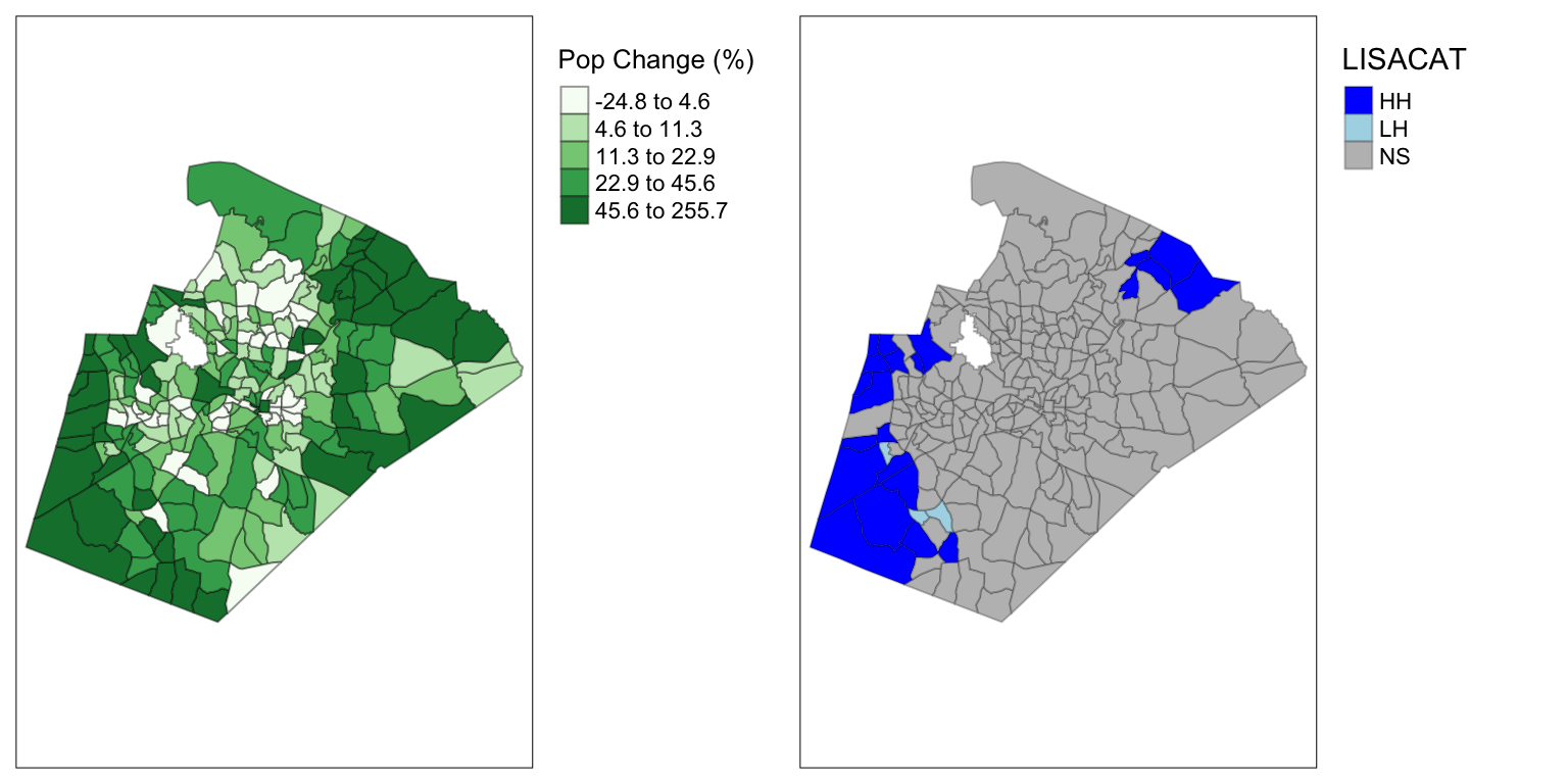
Code
Click here to download the R code from this module
This page was last updated on February 26, 2024